Christmas Storm of 1811

See also

Video version

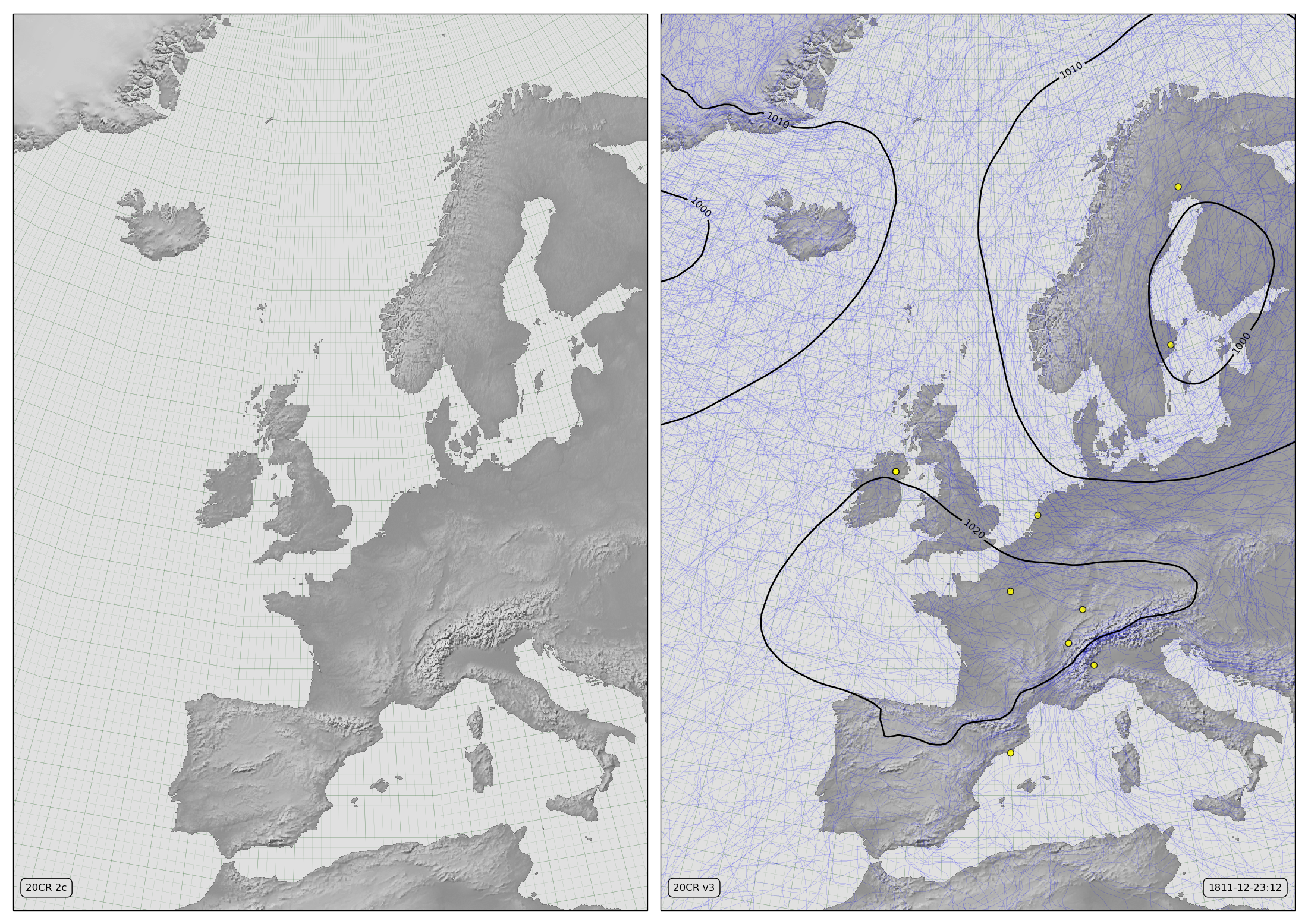
MSLP for v3 (right) - there is no v2c data for 1811.

The thin blue lines are mslp contours from the first 56 ensemble members . The thicker black lines are contours of the ensemble mean. The yellow dots mark pressure observations assimilated while making the field shown.

The Christmas storm of 1811 Drove HMS Defence, HMS St George, HMS Hero, and HMS Grasshopper aground on Jutland: more than 1,900 sailors were killed.

This means strong north-west winds in the north sea, and implies a deep low over scandinavia. The uncertainties are large, which reduces the amplitude of the ensemble mean signal, but 20CRv3 does reproduce this feature.

Code to make the figure

Download the data required:

#!/usr/bin/env python

import IRData.twcr as twcr
import datetime

dte=datetime.datetime(1811,12,1)
for version in (['4.5.1']):
    twcr.fetch('prmsl',dte,version=version)
    twcr.fetch_observations(dte,version=version)

Make the figure:

#!/usr/bin/env python

# UK region weather plot 
# Compare pressures from 20CRV3 and 20CRV2c

import math
import datetime
import numpy
import pandas

import iris
import iris.analysis

import matplotlib
from matplotlib.backends.backend_agg import \
             FigureCanvasAgg as FigureCanvas
from matplotlib.figure import Figure

import cartopy
import cartopy.crs as ccrs

import Meteorographica as mg
import IRData.twcr as twcr

# Date to show
year=1811
month=12
day=23
hour=12
dte=datetime.datetime(year,month,day,hour)

# Landscape page
fig=Figure(figsize=(22,22/math.sqrt(2)),  # Width, Height (inches)
           dpi=100,
           facecolor=(0.88,0.88,0.88,1),
           edgecolor=None,
           linewidth=0.0,
           frameon=False,
           subplotpars=None,
           tight_layout=None)
canvas=FigureCanvas(fig)

# UK-centred projection
projection=ccrs.RotatedPole(pole_longitude=180, pole_latitude=35)
scale=15
extent=[scale*-1,scale,scale*-1*math.sqrt(2),scale*math.sqrt(2)]

# Two side-by-side plots
ax_2c=fig.add_axes([0.01,0.01,0.485,0.98],projection=projection)
ax_2c.set_axis_off()
ax_2c.set_extent(extent, crs=projection)
ax_3=fig.add_axes([0.505,0.01,0.485,0.98],projection=projection)
ax_3.set_axis_off()
ax_3.set_extent(extent, crs=projection)

# Background, grid and land for both
ax_2c.background_patch.set_facecolor((0.88,0.88,0.88,1))
ax_3.background_patch.set_facecolor((0.88,0.88,0.88,1))
mg.background.add_grid(ax_2c)
mg.background.add_grid(ax_3)
land_img_2c=ax_2c.background_img(name='GreyT', resolution='low')
land_img_3=ax_3.background_img(name='GreyT', resolution='low')


# 20CR2c label
mg.utils.plot_label(ax_2c,'20CR 2c',
                     facecolor=fig.get_facecolor(),
                     x_fraction=0.02,
                     horizontalalignment='left')

# V3 panel

# Add the observations from v3
obs=twcr.load_observations_fortime(dte,version='4.5.1')
mg.observations.plot(ax_3,obs,radius=0.15)

# load the V3 pressures
prmsl=twcr.load('prmsl',dte,version='4.5.1')

# Contour spaghetti plot of ensemble members
# Only use 56 members to match v2c
prmsl_r=prmsl.extract(iris.Constraint(member=list(range(0,56))))
mg.pressure.plot(ax_3,prmsl_r,scale=0.01,type='spaghetti',
                   resolution=0.25,
                   levels=numpy.arange(870,1050,10),
                   colors='blue',
                   label=False,
                   linewidths=0.1)

# Add the ensemble mean - with labels
prmsl_m=prmsl.collapsed('member', iris.analysis.MEAN)
mg.pressure.plot(ax_3,prmsl_m,scale=0.01,
                   resolution=0.25,
                   levels=numpy.arange(870,1050,10),
                   colors='black',
                   label=True,
                   linewidths=2)

mg.utils.plot_label(ax_3,'20CR v3',
                     facecolor=fig.get_facecolor(),
                     x_fraction=0.02,
                     horizontalalignment='left')

mg.utils.plot_label(ax_3,
              '%04d-%02d-%02d:%02d' % (year,month,day,hour),
              facecolor=fig.get_facecolor(),
              x_fraction=0.98,
              horizontalalignment='right')

# Output as png
fig.savefig('V3only_x11_%04d%02d%02d%02d.png' % 
                                  (year,month,day,hour))