Validation Spread v. Error plot January 1872 + Spring 1903 + February 1953
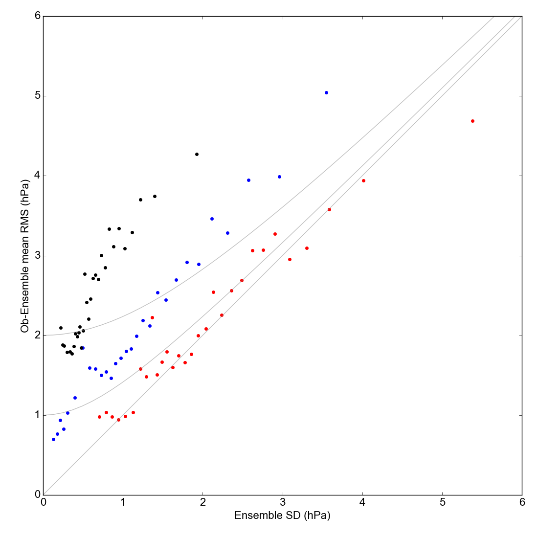
RMS reanalysis difference from observations, against reanalysis spread. For three reanalyses: 20CR2c in black, 20CR3 in red, and CERA-20C in blue.
The comparison includes data from three months of January to March 1903, augmented by January 1872 (higher spread) and Febriuary 1953 (lower spread).
If the observations were perfect, and the reanalysis spread was an unbiased estimate of its error, the RMS difference and the spread would be the same at all points. Because the observations have error, the RMS difference should be bigger than the spread, especially at small spread: the three grey lines show the expected relationship for three values of observation error (0, 1 and 2hPa). If the points are above the lines, the reanalysis is overconfident (spread too small) - if they are below the lines it is underconfident (spread too large).
First make the equivalent figure for each period seperately:
Then make the figure
#!/usr/bin/env python

# Scatter plot of reanalysis spread v reanalysis error
#  comparing three reanalyses

import os
import pickle
import datetime

import matplotlib
from matplotlib.backends.backend_agg import \
                 FigureCanvasAgg as FigureCanvas
from matplotlib.figure import Figure

import DWR_plots

start=datetime.datetime(1871,1,1)
end  =datetime.datetime(1953,4,1)

# Landscape page
fig=Figure(figsize=(11,11),  # Width, Height (inches)
           dpi=100,
           facecolor=(0.88,0.88,0.88,1),
           edgecolor=None,
           linewidth=0.0,
           frameon=False,
           subplotpars=None,
           tight_layout=None)
canvas=FigureCanvas(fig)
font = {'family' : 'sans-serif',
        'sans-serif' : 'Arial',
        'weight' : 'normal',
        'size'   : 16}
matplotlib.rc('font', **font)

# load the data for one reanalysis
def loadr(reanalysis):
    ddir=("%s/images/DWR/reanalysis_comparison_%s" %
                    (os.getenv('SCRATCH'),reanalysis))
    cdata={'ensembles':[],'observations':[]}
    dfiles=os.listdir(ddir)
    for dfl in dfiles:
       fdate=datetime.datetime(int(dfl[0:4]),int(dfl[5:7]),
                               int(dfl[8:10]),int(dfl[11:13]),
                               int(dfl[14:16]))
       if fdate<start or fdate >= end: continue
       d_file = open("%s/%s" % (ddir,dfl), 'rb')
       dpoint = pickle.load(d_file)
       d_file.close()
       cdata['ensembles']=cdata['ensembles']+dpoint['ensembles']
       cdata['observations']=cdata['observations']+dpoint['observations']
    return cdata

# Fill the frame with an axes
ax=fig.add_axes([0.08,0.08,0.89,0.89])

dmonth = loadr('cera')
DWR_plots.plot_eve(ax,dmonth,point_color=(0,0,1),nbins=30)

dmonth = loadr('20cr2c')
DWR_plots.plot_eve(ax,dmonth,obs_errors=None,point_color=(0,0,0),nbins=30)

dmonth = loadr('20cr3')
DWR_plots.plot_eve(ax,dmonth,obs_errors=None,point_color=(1,0,0),nbins=30)


# Output as png
fig.savefig('E_v_E.png')