South American cold surge of 2005 video
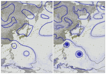
The thin lines are MSLP contours from each of 56 ensemble members. The thicker lines are contours of the ensemble mean. The background colour field shows the ensemble mean temperature at 850hPa. The small circles mark pressure observations assimilated while making the fields shown.
Code to make the figure
Download the data required:
#!/usr/bin/env python

import IRData.twcr as twcr
import datetime

dte=datetime.datetime(2005,9,1)

twcr.fetch('observations',dte,version='4.5.2')
twcr.fetch('prmsl',dte,version='4.5.2')
twcr.fetch('tmp',dte,level=850,version='4.5.2')

twcr.fetch('observations',dte,version='2c')
twcr.fetch('prmsl',dte,version='2c')
twcr.fetch('t850',dte,version='2c')
Script to make an individual frame - takes year, month, day, and hour as command-line options:
#!/usr/bin/env python

# South America plot
# MSLP and 850hPa temperature from 20CRv3 and v2c

import os
import math
import datetime
import numpy
import pandas

import iris
import iris.analysis

import matplotlib
from matplotlib.backends.backend_agg import \
             FigureCanvasAgg as FigureCanvas
from matplotlib.figure import Figure

import cartopy
import cartopy.crs as ccrs

import Meteorographica as mg
import IRData.twcr as twcr

# Fix dask SPICE bug
import dask
dask.config.set(scheduler='single-threaded')

# Get the datetime to plot from commandline arguments
import argparse
parser = argparse.ArgumentParser()
parser.add_argument("--year", help="Year",
                    type=int,required=True)
parser.add_argument("--month", help="Integer month",
                    type=int,required=True)
parser.add_argument("--day", help="Day of month",
                    type=int,required=True)
parser.add_argument("--hour", help="Time of day (0 to 23.99)",
                    type=float,required=True)
parser.add_argument("--opdir", help="Directory for output files",
                    default="%s/images/SA_cold_surge_2005" % \
                                           os.getenv('SCRATCH'),
                    type=str,required=False)
args = parser.parse_args()
if not os.path.isdir(args.opdir):
    os.makedirs(args.opdir)

dte=datetime.datetime(args.year,args.month,args.day,
                      int(args.hour),int(args.hour%1*60))

# HD video size 1920x1080
aspect=16.0/9.0
fig=Figure(figsize=(10.8*aspect,10.8),  # Width, Height (inches)
           dpi=100,
           facecolor=(0.88,0.88,0.88,1),
           edgecolor=None,
           linewidth=0.0,
           frameon=False,
           subplotpars=None,
           tight_layout=None)
canvas=FigureCanvas(fig)

# South America-centred projection
projection=ccrs.RotatedPole(pole_longitude=120, pole_latitude=125)
scale=30
extent=[scale*-1*aspect/2,scale*aspect/2,scale*-1,scale]

# Two side-by-side plots
ax_2c=fig.add_axes([0.01,0.01,0.485,0.98],projection=projection)
ax_2c.set_axis_off()
ax_2c.set_extent(extent, crs=projection)
ax_3=fig.add_axes([0.505,0.01,0.485,0.98],projection=projection)
ax_3.set_axis_off()
ax_3.set_extent(extent, crs=projection)

# Background, grid and land for both
ax_2c.background_patch.set_facecolor((0.88,0.88,0.88,1))
ax_3.background_patch.set_facecolor((0.88,0.88,0.88,1))
mg.background.add_grid(ax_2c)
mg.background.add_grid(ax_3)
land_img_2c=ax_2c.background_img(name='GreyT', resolution='low')
land_img_3=ax_3.background_img(name='GreyT', resolution='low')

# Observations
obs=twcr.load_observations_fortime(dte,version='2c')
obs=obs.loc[((obs['Latitude']<10) &
                 (obs['Latitude']>-90)) &
              ((obs['Longitude']>270) &
                 (obs['Longitude']<330))].copy()
mg.observations.plot(ax_2c,obs,radius=0.15)

# MSLP
prmsl=twcr.load('prmsl',dte,version='2c')

# Contour spaghetti plot of MSLP ensemble
mg.pressure.plot(ax_2c,prmsl,scale=0.01,type='spaghetti',
                   resolution=0.25,
                   levels=numpy.arange(870,1050,10),
                   colors='grey',
                   label=False,
                   linewidths=0.1,
                   zorder=150)

# Add the ensemble mean - with labels
prmsl_m=prmsl.collapsed('member', iris.analysis.MEAN)
mg.pressure.plot(ax_2c,prmsl_m,scale=0.01,
                   resolution=0.25,
                   levels=numpy.arange(870,1050,10),
                   colors='grey',
                   label=False,
                   linewidths=2,
                   zorder=200)

# Show the ensemble mean T850 with a colour overlay
t850=twcr.load('t850',dte,version='2c')
t850_m=t850.collapsed('member', iris.analysis.MEAN)
mg.precipitation.plot(ax_2c,t850_m,resolution=0.25,sqrt=False,
                      cmap=matplotlib.cm.get_cmap('coolwarm'),
                      vmin=265,vmax=295,alpha=0.5,zorder=100)

mg.utils.plot_label(ax_2c,'20CRv2c',
                     facecolor=fig.get_facecolor(),
                     x_fraction=0.02,
                     horizontalalignment='left',
                     zorder=500)

# V3 version
obs=twcr.load_observations_fortime(dte,version='4.5.2')
obs=obs.loc[((obs['Latitude']<10) &
                 (obs['Latitude']>-90)) &
              ((obs['Longitude']>270) &
                 (obs['Longitude']<330))].copy()
mg.observations.plot(ax_3,obs,radius=0.15)

# MSLP
prmsl=twcr.load('prmsl',dte,version='4.5.2')

# Contour spaghetti plot of MSLP ensemble
mg.pressure.plot(ax_3,prmsl,scale=0.01,type='spaghetti',
                   resolution=0.25,
                   levels=numpy.arange(870,1050,10),
                   colors='grey',
                   label=False,
                   linewidths=0.2,
                   zorder=150)

# Add the ensemble mean - with labels
prmsl_m=prmsl.collapsed('member', iris.analysis.MEAN)
mg.pressure.plot(ax_3,prmsl_m,scale=0.01,
                   resolution=0.25,
                   levels=numpy.arange(870,1050,10),
                   colors='grey',
                   label=False,
                   linewidths=2,
                   zorder=200)

# Show the ensemble mean T850 with a colour overlay
t850=twcr.load('tmp',dte,level=850,version='4.5.2')
t850_m=t850.collapsed('member', iris.analysis.MEAN)
mg.precipitation.plot(ax_3,t850_m,resolution=0.25,sqrt=False,
                      cmap=matplotlib.cm.get_cmap('coolwarm'),
                      vmin=265,vmax=295,alpha=0.5,zorder=100)

mg.utils.plot_label(ax_3,'20CRv3',
                     facecolor=fig.get_facecolor(),
                     x_fraction=0.02,
                     horizontalalignment='left',
                     zorder=500)

mg.utils.plot_label(ax_3,
              '%04d-%02d-%02d:%02d' % (args.year,args.month,
                                       args.day,int(args.hour)),
              facecolor=fig.get_facecolor(),
              x_fraction=0.98,
              horizontalalignment='right',
              zorder=500)

# Output as png
fig.savefig('%s/CS_V3vV2c_%04d%02d%02d%02d%02d.png' %
               (args.opdir,args.year,args.month,args.day,
                           int(args.hour),int(args.hour%1*60)))
To make the video, it is necessary to run the script above hundreds of times - giving an image for every 15-minute period. This script makes the list of commands needed to make all the images, which can be run in parallel.
#!/usr/bin/env python

# Make all the individual frames for a movie

import os
import subprocess
import datetime

# Where to put the output files
opdir="%s/slurm_output" % os.getenv('SCRATCH')
if not os.path.isdir(opdir):
    os.makedirs(opdir)

# Function to check if the job is already done for this timepoint
def is_done(year,month,day,hour):
    op_file_name=("%s/images/SA_cold_surge_2005/" +
                  "CS_V3vV2c_%04d%02d%02d%02d%02d.png") % (
                            os.getenv('SCRATCH'),
                            year,month,day,int(hour),
                                        int(hour%1*60))
    if os.path.isfile(op_file_name):
        return True
    return False

f=open("run.txt","w+")

start_day=datetime.datetime(2005,  9, 10, 0)
end_day  =datetime.datetime(2005,  9, 18, 23)

current_day=start_day
while current_day<=end_day:
    for fraction in (0,.25,.5,.75):
        if is_done(current_day.year,current_day.month,
                       current_day.day,current_day.hour+fraction):
            continue
        cmd=("./CS_V3vV2c.py --year=%d --month=%d" +
            " --day=%d --hour=%f \n") % (
               current_day.year,current_day.month,
               current_day.day,current_day.hour+fraction)
        f.write(cmd)
    current_day=current_day+datetime.timedelta(hours=1)
f.close()
To turn the thousands of images into a movie, use ffmpeg
ffmpeg -r 24 -pattern_type glob -i SA_cold_surge_2005/\*.png \
       -c:v libx264 -threads 16 -preset slow -tune animation \
       -profile:v high -level 4.2 -pix_fmt yuv420p -crf 25 \
       -c:a copy SA_cold_surge_2005.mp4