Princesse Alice II Expedition (1898): Pressure observations

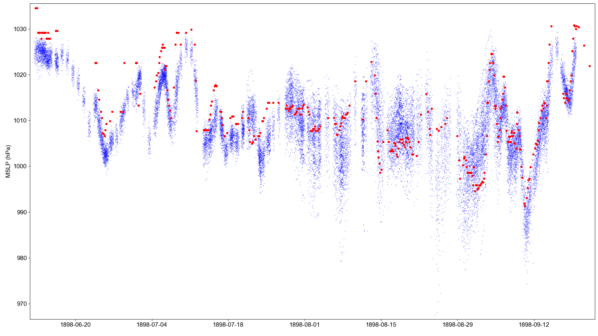
Atmospheric pressure observations made by the Princesse Alice II (red dots), compared with co-located MSLP in the 20CRv3 ensemble (blue dots).

Get the 20CRv3 data for comparison:

import IRData.twcr as twcr
import datetime

dtn=datetime.datetime(1898,1,1)
twcr.fetch('PRMSL',dtn,version='3')

Extract 20CRv3 MSLP at the time and place of each IMMA record. Uses this script:

./get_comparators.py --imma=../../../imma/Princess_Alice_II_1898.imma --var=PRMSL

Make the figure:

#!/usr/bin/env python

# Plot a comparison of a set of ship obs against 20CRv3

# Requires 20CR data to have already been extracted with get_comparators.py

obs_file='../../../../imma/Princesse_Alice_II_1898.imma'
pickled_20CRdata_file='20CRv3_PRMSL.pkl'

import pickle
import IMMA
import datetime
import numpy

import matplotlib
from matplotlib.backends.backend_agg import \
                 FigureCanvasAgg as FigureCanvas
from matplotlib.figure import Figure

# Load the data to plot
obs=IMMA.read(obs_file)
rdata=pickle.load(open(pickled_20CRdata_file,'rb'))
ob_dates=([datetime.datetime(o['YR'],o['MO'],o['DY'],int(o['HR'])) 
                  for o in obs if 
                (o['YR'] is not None and
                 o['MO'] is not None and
                 o['DY'] is not None and
                 o['HR'] is not None)])
ob_values=[o['SLP'] for o in obs if o['SLP'] is not None]
rdata_values=[value/100.0 for ensemble in rdata for value in ensemble[3]]

# Set up the plot
aspect=16.0/9.0
fig=Figure(figsize=(10.8*aspect,10.8),  # Width, Height (inches)
           dpi=100,
           facecolor=(0.88,0.88,0.88,1),
           edgecolor=None,
           linewidth=0.0,
           frameon=False,
           subplotpars=None,
           tight_layout=None)
canvas=FigureCanvas(fig)
font = {'family' : 'sans-serif',
        'sans-serif' : 'Arial',
        'weight' : 'normal',
        'size'   : 14}
matplotlib.rc('font', **font)

# Single axes - var v. time
ax=fig.add_axes([0.05,0.05,0.945,0.94])
# Axes ranges from data
ax.set_xlim((min(ob_dates)-datetime.timedelta(days=1),
             max(ob_dates)+datetime.timedelta(days=1)))
ax.set_ylim((min(min(ob_values),min(rdata_values))-1,
             max(max(ob_values),max(rdata_values))+1))
ax.set_ylabel('MSLP (hPa)')

# Ensemble values - one point for each member at each time-point
t_jitter=numpy.random.uniform(low=-6,high=6,size=len(rdata[0][3]))
for i in rdata:
    ensemble=numpy.array([v/100.0 for v in i[3]]) # in hPa
    dates=[i[0]+datetime.timedelta(hours=t) for t in t_jitter]
    ax.scatter(dates,ensemble,
                    10,
                    'blue', # Color
                    marker='.',
                    edgecolors='black',
                    linewidths=0.0,
                    alpha=0.5,
                    zorder=50)

# Observations
ob_dates=([datetime.datetime(o['YR'],o['MO'],o['DY'],int(o['HR'])) 
                  for o in obs if 
                (o['SLP'] is not None and
                 o['YR'] is not None and
                 o['MO'] is not None and
                 o['DY'] is not None and
                 o['HR'] is not None)])
ob_values=([o['SLP'] 
                  for o in obs if 
                (o['SLP'] is not None and
                 o['YR'] is not None and
                 o['MO'] is not None and
                 o['DY'] is not None and
                 o['HR'] is not None)])
ax.scatter(ob_dates,ob_values,
                100,
                'red', # Color
                marker='.',
                edgecolors='black',
                linewidths=0.0,
                alpha=1.0,
                zorder=100)
#ob_values_shifted=[value-12 for value in ob_values]
#ax.scatter(ob_dates,ob_values_shifted,
#                100,
#                'red', # Color
#                marker='.',
#                edgecolors='black',
#                linewidths=0.0,
#                alpha=1.0,
#                zorder=100)

fig.savefig('pressure_comparison.png')