Kon-Tiki Expedition (1947): Wind direction observations

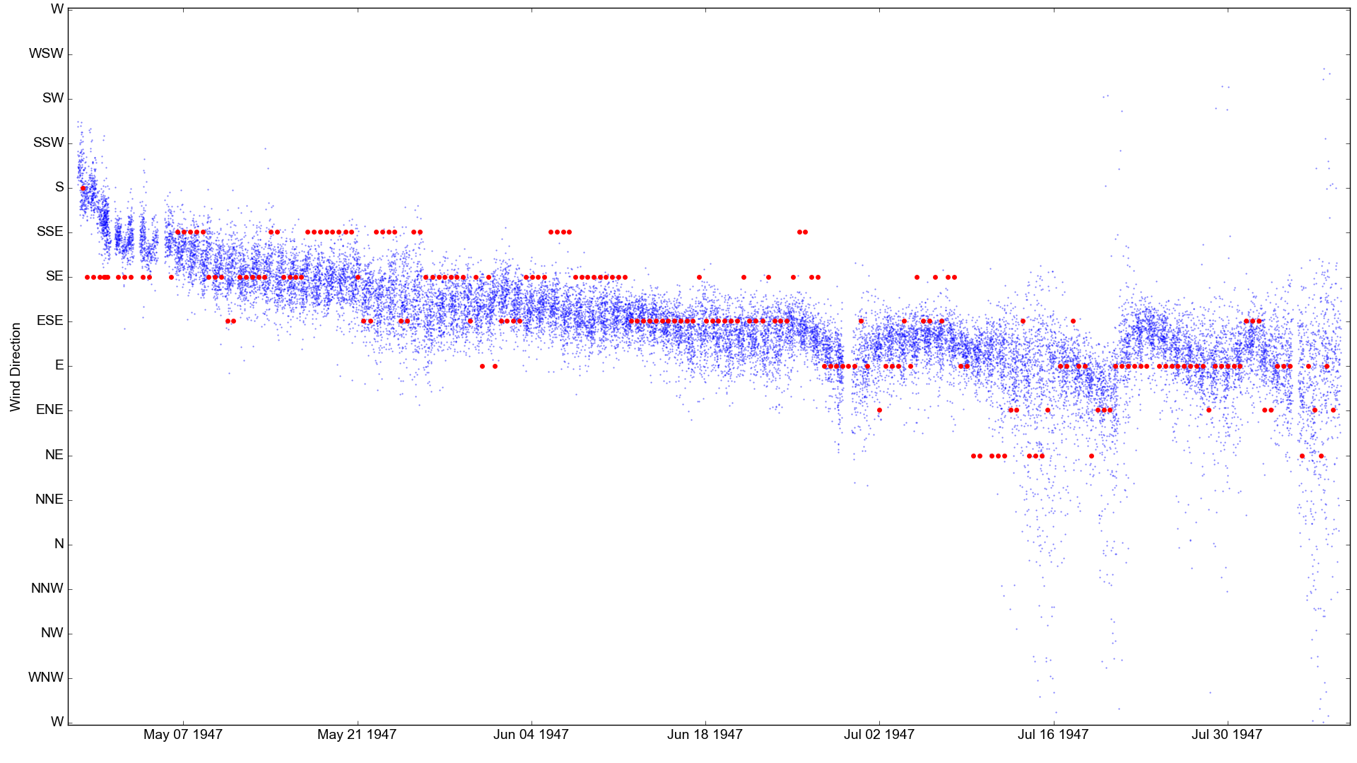
Wind direction observations made by the Kon-Tiki (red dots), compared with co-located 10m wind direction in the 20CRv3 ensemble (blue dots).

The observed wind directions are almost certainly magnetic. To convert them to true would mean adding about 7 degrees (1/3 point) - moving them up with respect to the reanalysis data.

The wind observations were made with a hand-held anemometer, probably at the masthead (maybe 6m above sea-level).

Get the 20CRv3 data for comparison:

import IRData.twcr as twcr
import datetime

for month in (4,5,6,7,8):
    dtn=datetime.datetime(1947,month,1)
    twcr.fetch('uwnd.10m',dtn,version='4.5.1')
    twcr.fetch('vwnd.10m',dtn,version='4.5.1')

Extract 20CRv3 10-metre zonal and meridional wind speeds at the time and place of each IMMA record. Uses this script:

./get_comparators.py --imma=../../../imma/Kon-Tiki_1947.imma --var=uwnd.10m
./get_comparators.py --imma=../../../imma/Kon-Tiki_1947.imma --var=vwnd.10m

Make the figure:

#!/usr/bin/env python

# Plot a comparison of a set of ship obs against 20CRv3

# Requires 20CR data to have already been extracted with get_comparators.py

obs_file='../../../../imma/Kon-Tiki_1947.imma'
pickled_20CRdata_file_u='20CRv3_uwnd.10m.pkl'
pickled_20CRdata_file_v='20CRv3_vwnd.10m.pkl'

import pickle
import IMMA
import datetime
import numpy
import math

import matplotlib
from matplotlib.backends.backend_agg import \
                 FigureCanvasAgg as FigureCanvas
from matplotlib.figure import Figure

# Load the data to plot
obs=IMMA.read(obs_file)
rdata_u=pickle.load(open(pickled_20CRdata_file_u,'rb'))
rdata_v=pickle.load(open(pickled_20CRdata_file_v,'rb'))
# Convert u and v to degrees from north
for i in range(len(rdata_u)):
    for j in range(len(rdata_u[i][3])):
        rdata_u[i][3][j]=((180.0/math.pi)*
                          math.atan2(rdata_v[i][3][j],rdata_u[i][3][j]*-1)
                          +90)

ob_dates=([datetime.datetime(o['YR'],o['MO'],o['DY'],int(o['HR'])) 
                  for o in obs if 
                (o['YR'] is not None and
                 o['MO'] is not None and
                 o['DY'] is not None and
                 o['HR'] is not None)])
ob_values=[o['W'] for o in obs if o['W'] is not None]
rdata_values=[value for ensemble in rdata_u for value in ensemble[3]]

# Set up the plot
aspect=16.0/9.0
fig=Figure(figsize=(10.8*aspect,10.8),  # Width, Height (inches)
           dpi=100,
           facecolor=(0.88,0.88,0.88,1),
           edgecolor=None,
           linewidth=0.0,
           frameon=False,
           subplotpars=None,
           tight_layout=None)
canvas=FigureCanvas(fig)
font = {'family' : 'sans-serif',
        'sans-serif' : 'Arial',
        'weight' : 'normal',
        'size'   : 14}
matplotlib.rc('font', **font)

# Single axes - var v. time
ax=fig.add_axes([0.05,0.05,0.945,0.94])
# Axes ranges from data
ax.set_xlim((min(ob_dates)-datetime.timedelta(days=1),
             max(ob_dates)+datetime.timedelta(days=1)))
ax.set_ylim((min(min(ob_values),min(rdata_values))-0.1,
             max(max(ob_values),max(rdata_values))+0.1))
ax.set_ylim(-91,271)
ax.yaxis.set_major_locator(
           matplotlib.ticker.FixedLocator(numpy.arange(-90,271,45/2.0)))
ax.yaxis.set_major_formatter(
           matplotlib.ticker.FixedFormatter(('W','WNW','NW','NNW','N','NNE','NE',
                                             'ENE','E','ESE','SE','SSE','S','SSW',
                                             'SW','WSW','W')))
ax.set_ylabel('Wind Direction')

# Ensemble values - one point for each member at each time-point
t_jitter=numpy.random.uniform(low=-6,high=6,size=len(rdata_u[0][3]))
for i in rdata_u:
    ensemble=numpy.array([v for v in i[3]]) # in hPa
    dates=[i[0]+datetime.timedelta(hours=t) for t in t_jitter]
    ax.scatter(dates,ensemble,
                    10,
                    'blue', # Color
                    marker='.',
                    edgecolors='black',
                    linewidths=0.0,
                    alpha=0.5,
                    zorder=50)

# Observations
ob_dates=([datetime.datetime(o['YR'],o['MO'],o['DY'],int(o['HR'])) 
                  for o in obs if 
                (o['D'] is not None and
                 o['YR'] is not None and
                 o['MO'] is not None and
                 o['DY'] is not None and
                 o['HR'] is not None)])
ob_values=([o['D'] 
                  for o in obs if 
                (o['D'] is not None and
                 o['YR'] is not None and
                 o['MO'] is not None and
                 o['DY'] is not None and
                 o['HR'] is not None)])
ax.scatter(ob_dates,ob_values,
                100,
                'red', # Color
                marker='.',
                edgecolors='black',
                linewidths=0.0,
                alpha=1.0,
                zorder=100)

fig.savefig('D_comparison.png')